Fading Glaciers: Where to Find the Path to Sustainability in Juneau?
Summary
In this paper, we develop a single-objective nonlinear planning model based on the coupled coordination degree for the sustainable tourism problem, which determines the proportion of excess to be allocated, and the basic conditions needed to achieve sustainable tourism.
For the optimization problem of sustainable tourism in Juneau City, we established a single-objective nonlinear planning model to determine the optimal solution. We established the model by taking the maximization of the coupling of social satisfaction index SI , environmental index EnI , and economical index EcI as the objective function, the number of tourists and the per capita tourism consumption as the decision variables, and the maximum capacity of tourists as the constraints.The main factors affecting SI were determined using principal component analysis-factor analysis, and the entropy weight method was used to determine the evaluation weights of the factors of EnI and the comprehensive evaluation index Tsuccessively, and the evaluation weights of the factors of T were used as the allocation ratio of the excess revenue among the factors. The relationship between EnI\&SIand the number of tourists and the average cost of tourism were obtained by regression fitting, and the coupling coordination model was introduced to find the best static solution through the interior point method. The future trend was predicted by the time series prediction method.The solution yields that excess revenue from tourism in Juneau is optimal when it is allocated according to economic aspects of 31.52%, environmental aspects of 19.36%, and social aspects of 49.12%.The coupling is maximized when the number of tourists reaches 1.175 million and the per capita tourism consumption increases by 2.98%. The trend for future development is that the overall tourism sustainable optimum can be achieved by 2027 through measures. Monte Carlo simulations using a simulation number of 100 were used to verify the global sensitivity, and it was found that there is a correlation effect between the number of tourists and the average tourist cost, leading to a greater impact of the average tourist cost on the degree of coordination than the number of tourists.
For Hawaii, a city with over-tourism, and Detroit, a city with the potential to develop tourism, we used our model to determine the optimal solution for the development of sustainable tourism in the two.According to the differences in the actual situation, we reasonably adjusted the determinants of the factors in the T, and calculated it. For Hawaii, the coupling degree reached the maximum value when the number of tourists reached 4.67 million, and the per capita tourism consumption decreased by about 3%; and for Detroit, when the tourist population reaches 2.5 million and the per capita tourism consumption decreases by about 5%, the coupling degree reaches the maximum value. This indicates the generalizability of our model.
Keywords:Principal Component Analysis-Factor Analysis, Entropy Weighting, Coupled Coordination Degree Model, Dynamic Programming, Monte Carlo Simulation
Contents
1 Introduction
1.1 Problem Background
1.2 Restatement of the Problem
1.3 Our Work
2 Notations
3 Assumptions and Justifications
4 Establishing the Coupling Coordination Model to Find the Optimal Tourism Equilibrium
4.1 Model Overview
4.2 Modeling of the Economical Index EcI(x, y)
4.3 Modeling of the Environmental Index EnI(x, y)
4.3.1 Model Building
4.3.2 Solving for Component Weights Using the Entropy Weight Method
4.4 Modeling of the Social Satisfaction Index SI(x, y)
4.4.1 Model Building
4.4.2 Significant Influences on SI(x, y) Using Principal Component Analysis
4.4.3 Solving for Component Weights Using the Entropy Weight Method
4.5 Modeling of the Coupling Degree Coordination
4.5.1 Fitting of Environmental Index EnI(x, y) and Social Satisfaction Index SI(x, y) with Respect to x, y
4.5.2 Introduction of Coupling Degree C and Coupling Coordination Degree-D
4.5.3 Calculate the Maximum Value of D(x, y) under the Constraints
4.6 Funding Plan and Impact of Role Based on the Coupled Coordination Model
4.7 Applying Models to Predict the Future of Juneau’s Tourism Industry
5 Sensitivity Analysis
5.1 Sensitivity Analysis Overview
5.2 Partial Sensitivity Analysis of the Function D(x, y) near the Point of Maximum Value
5.3 Global Sensitivity Analysis of the Function D(x, y) Based on Monte Carlo Simulation
5.4 Sensitivity Analysis Conclusions
6 Application of the Model: Optimizing Sustainable Tourism Plans in OtherWorld Tourist Cities
6.1 Hawaii with Over-tourism
6.2 Detroit with Prospects for Tourism Development
7 Model Evaluation
7.1 Strengths
7.2 Weeknesses
8 Conclusions
1. Introductions
1.1 Problem Background
At a time when the global tourism industry is booming, tourism activities bring huge economic benefits to various places. Still, it is undeniable that the phenomenon of over-tourism is becoming more and more prominent.
Take the example of Juneau, Alaska, USA, a city with only about 30,000 residents, which hosted 1.6 million cruise ship passengers in 2023. The influx of tourists has brought about US $ 375 million in revenue for Juneau, but it has also led to several problems: the city's infrastructure is under enormous pressure, drinking water supplies are tight, waste disposal is difficult, and local carbon emissions have risen significantly. In addition, the influx of tourists has strained housing resources and increased prices, affecting the lives of residents.
To make matters worse, the Mendenhall Glacier, a famous attraction in Juneau, is retreating at an alarming rate. Studies have shown that global warming is the main cause of glacier retreat, which is also exacerbated to some extent by increased carbon emissions from excessive tourism. The retreat of glaciers not only destroys local natural landscapes but also makes many locals worry that with the disappearance of glaciers, tourists and related income will also go with them.
Against this backdrop, we will use the city of Juneau as an example to explore a model of sustainable tourism development, and generalize the findings to the many regions around the world affected by over-tourism, to achieve long-term stable development of the tourism industry, while preserving natural and cultural resources and safeguarding the quality of life of residents.
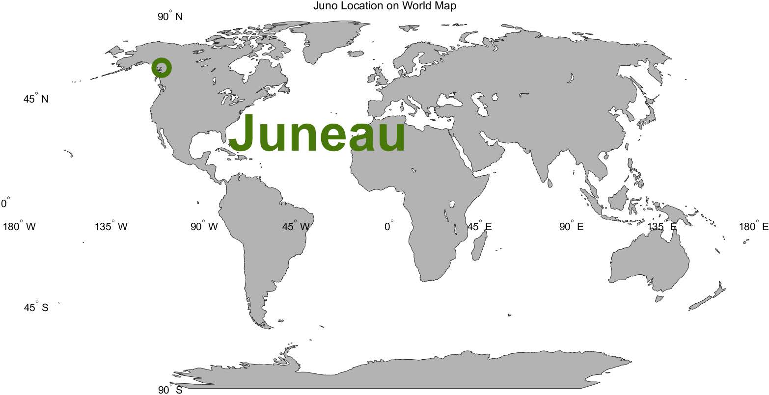
Figure 1: Geographic location of Juneau
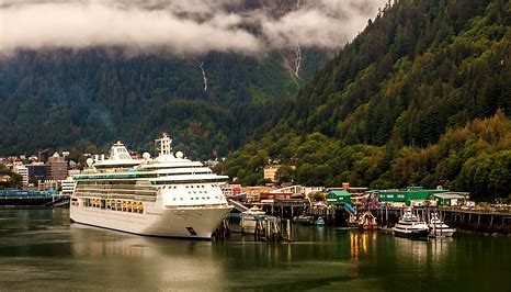
Figure 2: Cruises in Juneau
1.2 Restatement of the Problem
Considering the background information identified and the requirements given in the problem statement, we need to build a sustainable tourism model to determine, and solve the following problems:
Problem 1: Build an optimization model to regulate the tourism industry in the city of Juneau to a sustainable level, here we need to resolve the conflict between the environmental resource problem and the economic efficiency problem, balance the relationship between the two to reach a most appropriate level, and here we perform a sensitivity analysis to summarize the important factors that affect this model.
Problem 2: Adapt the model developed in the first task to another city that, like Juneau, is faced with adapting sustainable tourism development, and use the model to provide valuable, sustainable recommendations to help this city and discuss how the model can be applied to promote attractions or areas with fewer tourists. At the same time, another city with a low number of tourists is given reasonable suggestions for the development of tourism resources in order to attract tourists to develop tourism.
Problem 3: From the optimization conclusions of our model, provide advice to the City of Juneau to better inform the future direction of the City of Juneau.
1.3 Our work
In the coupled coordination degree modeling section (Blue Panels): We first determine the specific expression of the economical index according to the Juneau's tourism income and identify the main factors affecting social satisfaction index.Secondly, we determine the evaluation weights of the factors of the environmental index and the comprehensive evaluation index, then we determine the relationship between the environmental and social satisfaction indicators and the decision variables tourist arrivals and average cost of travel, and we find the best of their of the static program. Then we integrate the allocation of funds proportionally according to the weights of the components in the comprehensive evaluation indicators and test the rationality of the allocation results. Finally, we give recommendations for future policy development in the City of Juneau and predict trends in change.
In the sensitivity analysis section (Purple Panels): We analyze the local sensitivity and then study the global sensitivity to find out the decision variables that become the main influencing factors.
In the model application section (Light Green Panels): We selected Hawaii, which also suffers from over-tourism, and Detroit, a city that has the potential to develop tourism but is under-exploited, and we use our model to give recommendations for developing sustainable tourism.
The specific schematic is shown in figure3:
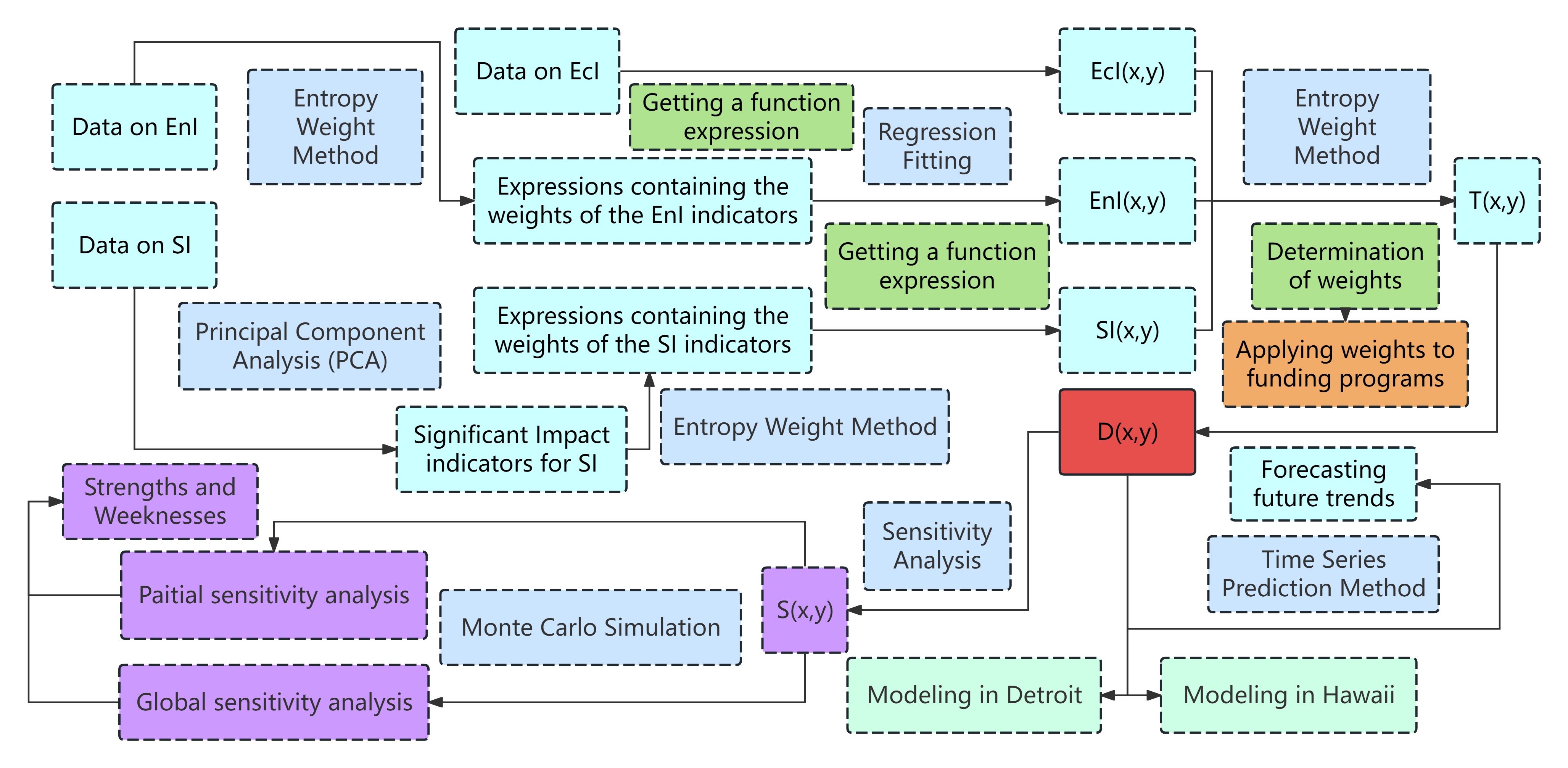
Figure 3: Our Work
2. Notations
| Symbol | Description | Unit |
|---|---|---|
| EnI(x, y) | Environmental Index | |
| EcI(x, y) | Economical Index | |
| SI(x, y) | Social Satisfaction Index | |
| T(x, y) | Comprehensive Evaluation Index | |
| C(x, y) | Coupling function | |
| D(x, y) | Harmonic function | |
| S(D, x) | D sensitivity to x | |
| S(D, y) | D sensitivity to y | |
| x | Percentage increase in travel costs | |
| y | Maximum number of visitors | |
| C e | Carbon emissions | t |
| C max | The maximum value of carbon emissions | t |
| C min | The minimum value of carbon emissions | t |
| C norm | Carbon emissions after data normalization | t |
| ωCe | The weighting of carbon emissions | |
| S g | Area of glaciers | m² |
| S max | The maximum value of the glacier area | m² |
| S min | The minimum value of the glacier area | m² |
| S norm | Area of glaciers after data normalization | m² |
| ωSg | The weighting of the glacier area | |
| X EcI(t) | The value of EcI at year t | |
| X EnI(t) | The value of EnI at year t | |
| X SI(t) | The value of SI at year t |
Note: There are some variables that are not listed here and will be discussed in detail in each section.
3. Assumptions and Justifications
• Assumption 1: In response to the predictions made using the model, this paper
argues that the number of tourists can reach the limited number of tourists after the
Juneau government has taken action, and the model replaces the actual number of
tourists with the maximum limited number of tourists.
• Justification 1:This is because the study of statistics found that in the post epidemic
era, the number of tourists has reached or even exceeded the pre-epidemic level, and
the number of tourist visitors showed a clear upward trend, and after the study, the
optimal number of tourists in the city of Juneau is smaller than the actual number
of tourists today.
• Assumption 2: The model assumes that the size and structure of the local resident
population (e.g., age, occupation, income level, etc.) will not change drastically over
the course of several years, and the fit in the model based on data from previous
years can be considered to maintain accuracy.
• Justification 2: Because Juneau is the capital of the State of Alaska, with a 145-
year history of cityhood and an average population growth rate of only 0.35 percent
between 2010 and 2020, the age structure of Juneau residents is relatively stable in
the 2020 Census report, and the job market is characterized by significant job market
characteristics, mostly in relatively stable industries such as tourism, fishing, and
resource development, which is unlikely to trigger large-scale demographic change.
• Assumption 3:The fitted relational equation remains constant before and after the
occurrence of external factors such as climatic extreme events, COVID-19, etc., when
partial data processing is carried out in the model.
• Justification 3:During the course of these external environmental influences, the
economy, society, environment, etc., changed considerably, but the data returned to
the right track some time after the event. Therefore the model is considered to be
valid within a manageable range.
4. Establishing the Coupling Coordination Model to Find the Optimal Tourism Equilibrium
4.1 Model Overview
In this model, we select percentage increase in travel costs as the decision variable x, maximum number of visitors as the decision variable y (tens of millions of people),establishing the comprehensive evaluation index T(x,y), and T(x,y) is related to the economical index EcI(x,y), the environmental index EnI(x,y) and social satisfaction index SI(x,y), and EcI(x,y), EnI(x,y),and SI(x,y) are all binary functions on x,y, respectively, so that T as a whole is also a binary function on x,y.
In the following, we will expand our discussion of EcI(x,y), EnI(x,y), and SI(x,y) by modeling and discussing these three subsections.(figure 4):
Figure 4: Schematic Diagram of the Coupling Degree Model
4.2 Modeling of the Economical Index EcI(x,y)
In the first aspect, we have modeled the economic aspect regarding the economical index EcI(x,y), where we define the economical index as the product of the number of tourists and the per capita consumption, from the previous section, the number of tourists after the restriction is y, and by querying the dataset, we can know the average consumption of tourists in the current case, C_0. Therefore, the economical index EcI(x,y), has the following expression:
4.3 Modeling of the Environmental Index EnI(x,y)
4.3.1 Model Building
In the second aspect, we modeled about the environmental index EnI(x,y) in the environmental dimension, according to the environmental report of Juneau City, we know that the environmental index of Juneau City can be measured by carbon emissions C_e and glacier area S_g, so we chose C_e and S_g as the important dimensions reflecting the environmental index EnI(x,y), and we obtained the expression of the environmental index EnI(x,y) with respect to x and y:
In the process of model solution, we first normalize the relevant data:
where, w_{C_e} is the weighting of carbon emissions, w_{S_g} is the weighting of the glacier length.
Then we use the entropy weighting method to find out the proportion of S_g and C_e in the environmental index EnI : w_{S_g}, w_{C_e}, respectively, and determine the value of the final environmental index EnI between 2016 and 2023
The following table shows the calculation process and results for each year:
| Year | ( S g ) | ( C e ) | ( S norm) | ( C norm ) | ( EnI ) |
|---|---|---|---|---|---|
| 2023 | 22.11 | 20.7 | 0.083 | 0.112 | 0.097 |
| 2022 | 25.57 | 21.1 | 0.096 | 0.114 | 0.105 |
| 2021 | 28.90 | 21.9 | 0.108 | 0.118 | 0.113 |
| 2020 | 32.11 | 22.7 | 0.120 | 0.123 | 0.121 |
| 2019 | 35.19 | 23.5 | 0.132 | 0.127 | 0.129 |
| 2018 | 38.14 | 24.3 | 0.143 | 0.131 | 0.137 |
| 2017 | 40.98 | 25.1 | 0.154 | 0.136 | 0.145 |
| 2016 | 43.70 | 25.9 | 0.164 | 0.140 | 0.152 |
4.3.2 Solving for Component Weights Using the Entropy Weight Method
Main steps of the entropy weighting method:
Data normalization: the indicators are de-measured to make them comparable.(table1)
Calculate the ratio of each indicator under each program: calculate the proportion of the value taken in each year to the total value.(equation4)
Find the information entropy of each indicator: calculate the information entropy of each indicator according to the definition of information entropy.(equation 5)
Determine the weight of each indicator: calculate the weight of each indicator according to the information entropy.(equation 6)
where,p_{ij} is the proportion of each indicator in each year,y_{ij} is the value of thej-th indicator in thei-th year,E_j is the information entropy of each indicator,n is the number of years,m is the number of indicators,w_j is the weight of each indicator.
The calculations show that:
Bringing in the expression forEnI (equation 2) yields:
4.4 Modeling of the Social Satisfaction IndexSI(x,y)
4.4.1 Model Building
In the third aspect, we modeled social satisfaction index at the social level. Since social satisfaction index is related to several factors, to facilitate the analysis of the results, we selected some of the most relevant factors from the information provided in the data set, such as the personal income of the population, the cost of living of the population, the price of housing, the poverty rate of the population and the unemployment rate.
Then, to easily characterize social satisfaction index, we have collected the economic conditions of the City of Juneau for the years 2016-2023 ( as shown in figure 5)and have used Principal Component Analysis - Factor Analysis to effectively solve this problem. ( equation 8)
4.4.2 Significant Influences onSI(x,y)
In order to easily characterize the social satisfaction index of the residents, we used Principal Component Analysis-Factor Analysis to solve this problem effectively. Since different attributes are good or bad for the results, for negative indicators such as the cost of living index, poverty rate, unemployment rate, and house price, we use the normalization process and take the negative number to get a new column of data.( figure 6)
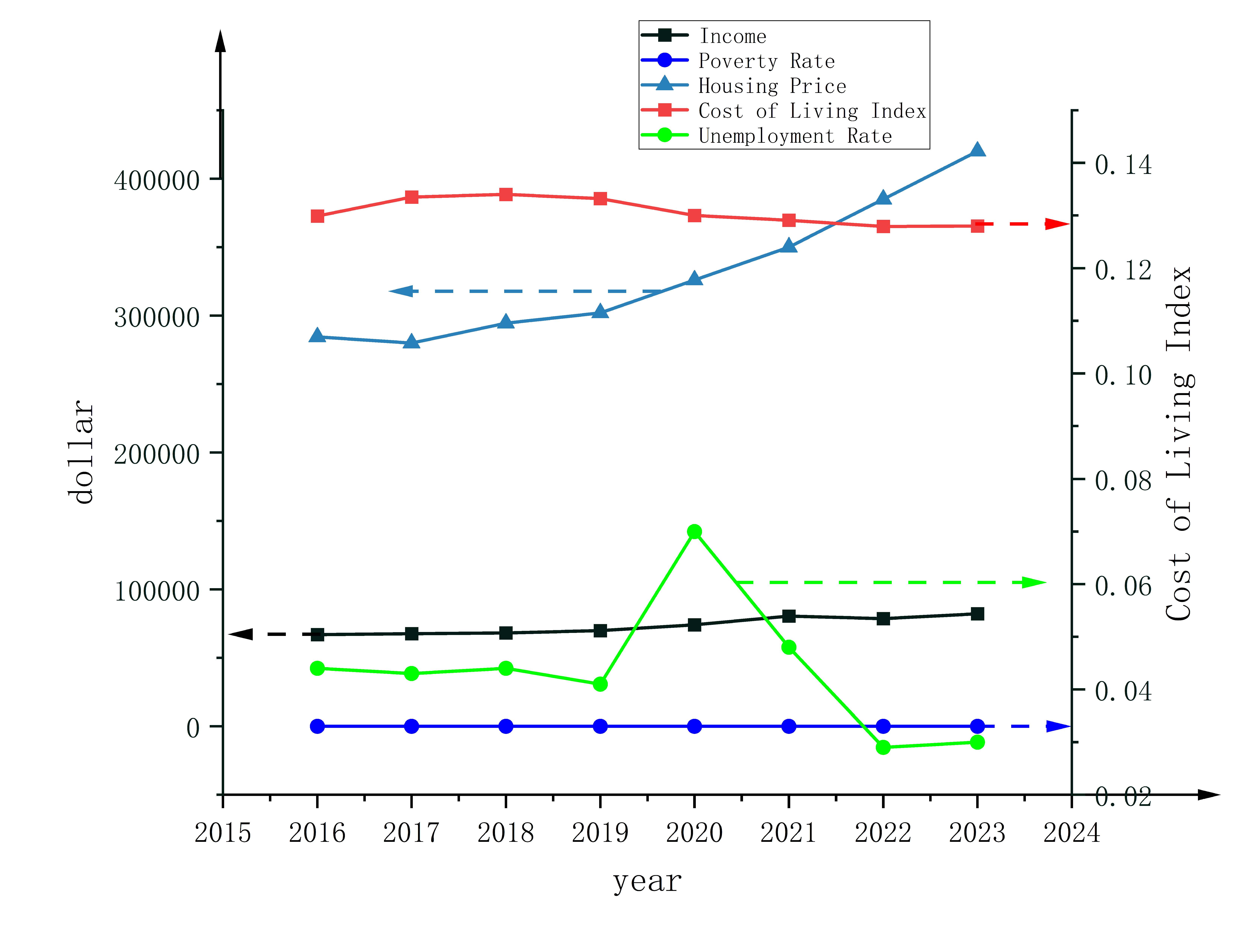
Figure 5: Data of Various Social Indicators
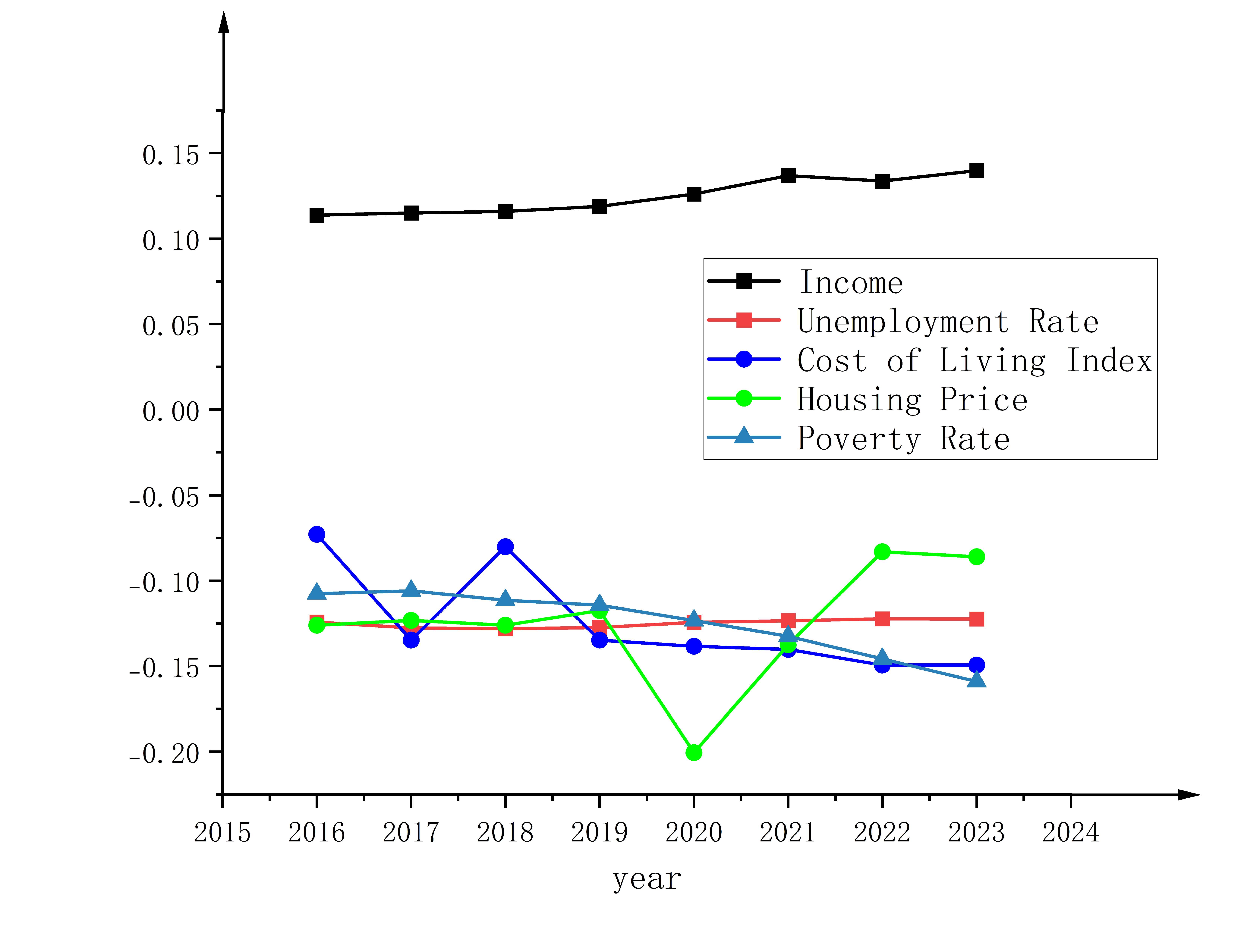
Figure 6: Data of Various Social Indicators
after Normalization
The absolute value of the result after weighted summation is proportional to social satisfaction indexSI(x,y).
where,a_{1i},a_{2i}\cdots a_{pi} (i =1,2,3 \cdots m) are the eigenvectors corresponding to the eigenvalues of the covariance matrix\Sigma of the matrixX,x_1,x_2 \cdots x_p are the values of the original variables, considering the data after normalization without considering the effect of magnitude. We first calculated the correlation coefficient matrix of this8\times5 matrix and then calculated its five eigenroots as:
We find that:
i.e. the two components, house price and unemployment rate, take up more than 80\% of the total components, so we can conclude that social satisfaction index is to some extent related to house price and unemployment rate only. By eliminating the other three evaluation attributes with lower weights and keeping these two, we finally recalculate the weight relationship between\lambda_4 and\lambda_5:
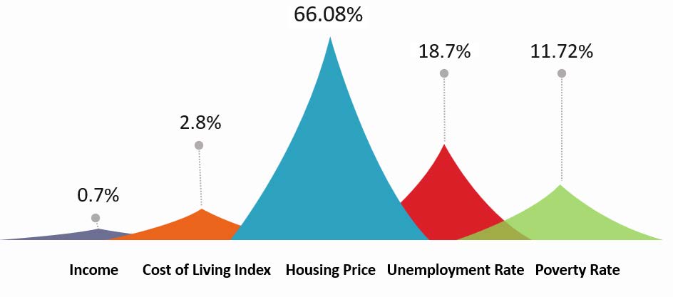
Figure 7: Percentage of the influencing factors for the social satisfaction indicator
Finally we calculated its social satisfaction indexSI year by year.(table 2)
Table 2: Original Data and Normalized Data (2016-2023)
| Year | Ecl | EnI | S | Year | Ecl | EnI | S | |
|---|---|---|---|---|---|---|---|---|
| ==> | ||||||||
| 2023 | 2387533 | 0.097 | 0.2117 | ==> | 2023 | 0.000 | 0.00 | 0.143 |
| 2022 | 2423728 | 0.105 | 0.2120 | ==> | 2022 | 0.167 | 0.27 | 0.132 |
| 2021 | 2421944 | 0.113 | 0.2078 | ==> | 2021 | 0.159 | 0.56 | 0.134 |
| 2020 | 2292657 | 0.121 | 0.2030 | ==> | 2020 | 0.000 | 0.83 | |
| 2019 | 2414435 | 0.129 | 0.2094 | ==> | 2019 | 0.146 | 1.00 | 0.115 |
| 2018 | 2467392 | 0.137 | 0.2087 | ==> | 2018 | 0.319 | 0.59 | 0.115 |
| 2017 | 2511152 | 0.145 | 0.2089 | ==> | 2017 | 0.500 | 0.59 | 0.110 |
| 2016 | 2437578 | 0.152 | 0.2087 | ==> | 2016 | 0.208 | 0.00 | 0.112 |
4.4.3 Solving for Component Weights Using the Entropy Weight Method
We define the comprehensive evaluation index as:
where,w_{EcI(x,y)},w_{EnI(x,y)},w_{SI(x,y)}, are weights, and they satisfy:
Following the previous section, we again use the entropy weighting method to find the weights of the components.
Through the calculation, we obtained the following weights:
Thus,the integrated optimization objective function is:
4.5 Modeling of the Coupling Degree Coordination
4.5.1 Fitting of Environmental Index EnI(x,y) and Social Satisfaction Index SI(x,y) with Respect to x,y
Knowing the weight coefficients of the ideal optimization model, we then determine the linear expression for the scientific determination of the ideal optimization model.
We have tabulated the results of the above calculations in the table 3. In which the number of tourists is measured in tens of millions due to the large number of tourists. ( indicates missing data)
Table 3:Data Used for Function Fitting
| Year | Enl | S | x | y |
|---|---|---|---|---|
| 2023 | 0.097 | 0.143 | / | 0.207 |
| 2022 | 0.105 | 0.132 | 0.006 | 0.156 |
| 2021 | 0.113 | 0.134 | 0.081 | 0.045 |
| 2020 | 0.121 | 0.140 | 0.049 | 0.028 |
| 2019 | 0.129 | 0.115 | -0.011 | 0.173 |
| 2018 | 0.137 | 0.115 | 0.014 | 0.115 |
| 2017 | 0.145 | 0.110 | 0.031 | 0.107 |
| 2016 | 0.152 | 0.112 | 0.005 | 0.102 |
First we determine the functional equation of the environmental indexEnI(x,y) withx,y. Since a decrease in the number of visiting tourists y is good for the environment and an increase in tourist travel expenses will limit the number of tourists, we can guess thaty inEnI(x,y) should be in the form of a similar inverse proportion or a negative exponent, and so we set:
( Pm(x) denotes a polynomial containing x), and fit each of the two functions using the relational equations in our table 3, excluding outliers due to COVID-19. We find the following regression equation 16, which has excellent coefficients of determination and confidence intervals.
Then we determine the relationship between social satisfaction index SI(x,y) and x,y. An increase in the average tourist fee leads to a higher income for residents but also to an increase in prices, so we fit a polynomial in x to this situation. An increase in the number of tourists can lead to conditions such as congestion, which can cause a bad experience for the residents and greatly reduce the social satisfaction index SI(x,y). So the following models were developed to fit the relationship:
and at last, we determined that the equation 19 characterizes the relationship well.(figure 9)
Ultimately we fit theEnI(x,y)andSI(x,y) tox, y, and ultimately obtain the expression ofT(x,y) as:
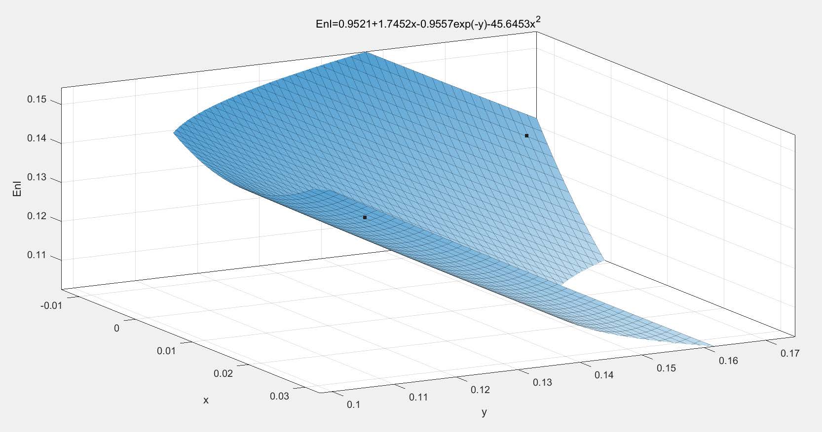
Figure 8: The Image of the Function Obtained after Fitting EnI(x, y)
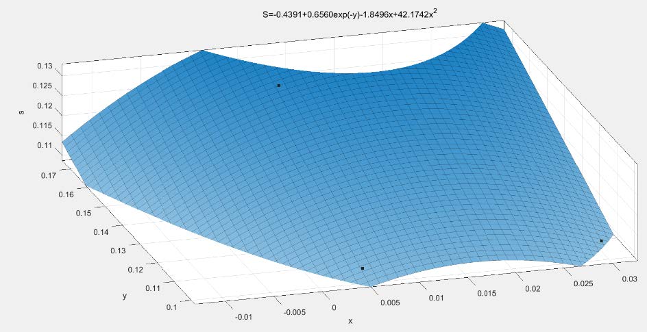
Figure 9: The Image of the Function Obtained after Fitting SI(x, y)
4.5.2 Introduction of Coupling Degree C and Coupling Coordination Degree D
Once we have obtained the mathematical expression T(x,y) for the total evaluation index, we use the expression to construct the coupling coordination degree model. The coupling coordination model is a common tool to measure the coupling relationship between systems, which can clearly portray the role of the relationship between systems, we can optimize the social level, environmental level, and tourism level influencing factors, find the best value of the decision variables, and come up with the most appropriate optimization plan and evaluation of the impact of the current measures through the establishment of this model.
After bringing in the simplification, we get the expression for D(x,y) as:
4.5.3 Calculate the Maximum Value of D(x, y) under the Constraints
For the above expression for D(x,y), we have some constraints: the maximum number of tourists is 16,000 per day and 12,000 on Saturdays, which is 5,632,000 per year.
where, y_{max} is annual maximum visitor capacity.
We use the fmincon function in MATLAB and the interior point method, iterating over and over to get the maximum point of D(x,y):
That is to say, if we increase total visitor spending by 2.98% over current levels through higher hotel taxes, higher alcohol sales, etc., and limit annual maximum visitor capacity to 1,174,700 visitors, we can achieve high quality, sustainable development in Juneau.
4.6 Funding Plan and Impact of Role Based on the Coupled Coordination Model
In the above model we determined the weights about EcI(x,y),EnI(x,y),SI(x,y) in the comprehensive evaluation index T(x,y). According to the weights of these three, we allocate the funding of additional income according to the weights to achieve the effect of the most significant rise in the comprehensive evaluation index T(x,y) in general.
According to equation 20, we first invest 19.36% of the funding in the economic aspects of tourism, and we invest these funds in infrastructure development to expand the scale of tourism and increase the quality and level of tourism services, which is conducive to the development of tourism in the long term.
In addition, we invested 31.52% of the funds in environmental protection, which we can use to improve glacier monitoring and protection, upgrade water resource management and urban drinking water systems, and build a carbon reduction and mitigation system to mitigate the environmental protection problems faced by the city of Juneau and increase the sustainability of ecotourism.
Finally, we invested 49.12% of the funds in building community programs to improve the sense of well-being of local residents through increased community communication and connections, and to provide social benefits to increase the acceptance of the region by local residents.
The distribution of funds is shown in figure 10:
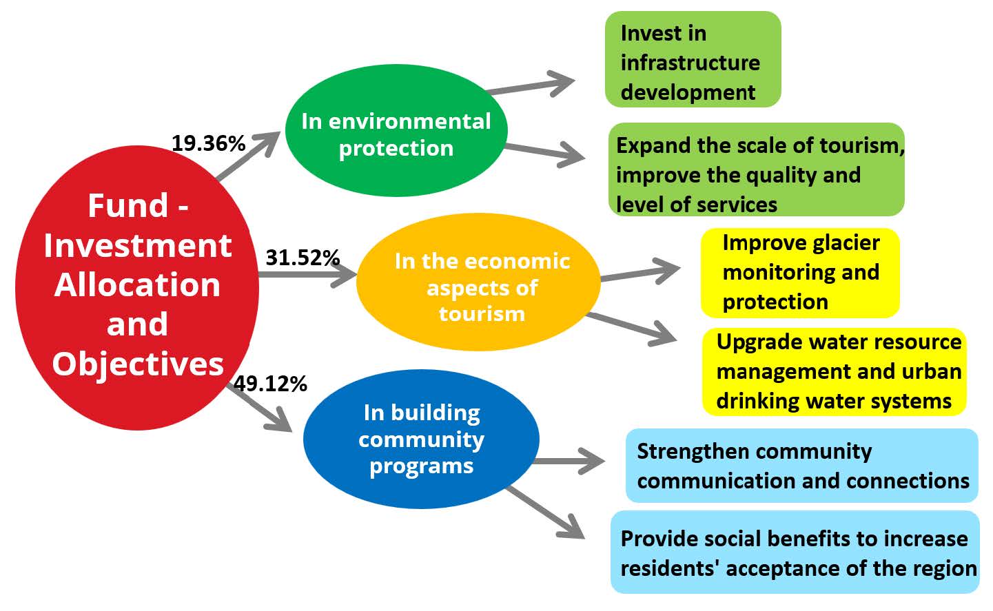
Figure 10: Funding Allocation Program
In the following, using our model to test the reasonableness of the above allocation, the following relationship exists between the relevant amount of change after allocation:
where,ΔEcI,ΔEnI, ΔSI, ΔD(x,y) are the amount of change in the value of EcI, EnI, SI, D(x,y) after investing funds.
After investing funds, according to our model, it was found that the value of D(x,y) increased after the realization of the distribution scheme, i.e., the coupling coordination increased and sustainable tourism was better developed.
4.7 Applying Models to Predict the Future of Juneau’s Tourism Industry
Above we use the fmincon interior point method to find x,y for the static optimal tourism consumption growth rate and the maximum number of tourists. In order to better reflect the effects of changes in these two variables on EcI,EnI, and SI, we built the following time-series prediction model. Definition X_{EcI}(t) denotes the value of EcI at year t. By the difference-by-difference method, we obtain an expression for \Delta X(EcI)(t) to evaluate the rate of change of this attribute:
and similarly we define \Delta X_{EnI}(t),\Delta X_{SI}(t). For the anomalies that occur in EcI,EnI, and SI over a period of time, we believe that the Juneau government can bring one of these values back to the right track by moderating x and restricting y. Obviously this value that is being The value that is adjusted should be the one with the smallest change, so we define the function:
At the same time, in order to ensure the normal functioning of public opinion and the economy of the city of Juneau, the variation of x,y should not exceed 10%, we calculate the maximum value of the abnormal indicator in this new interval through the dynamic programming algorithm, recognizing the x and y at this point in time and calculating the corresponding value of the corresponding other 2 indicators, thus predicting the data for the second year. Through continuous iteration, we ended up predicting a floating map of each indicator for the city of Juneau over a 5-year period in the presence of the corresponding policy.
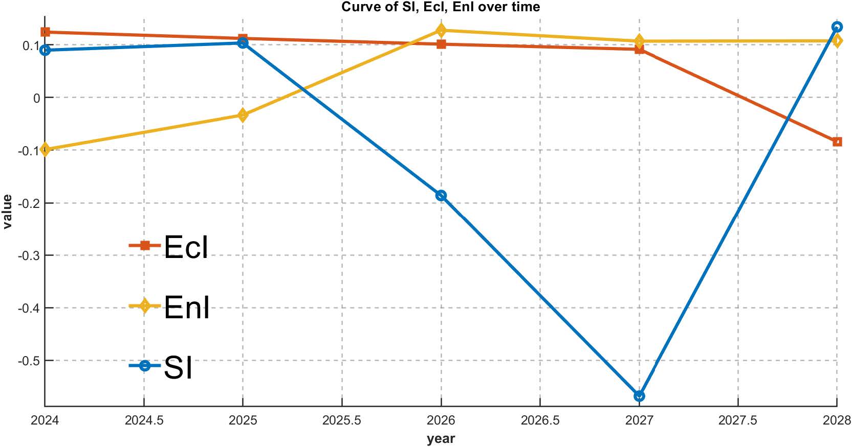
Figure 11: Curve of EcI,EnI, SI over Time
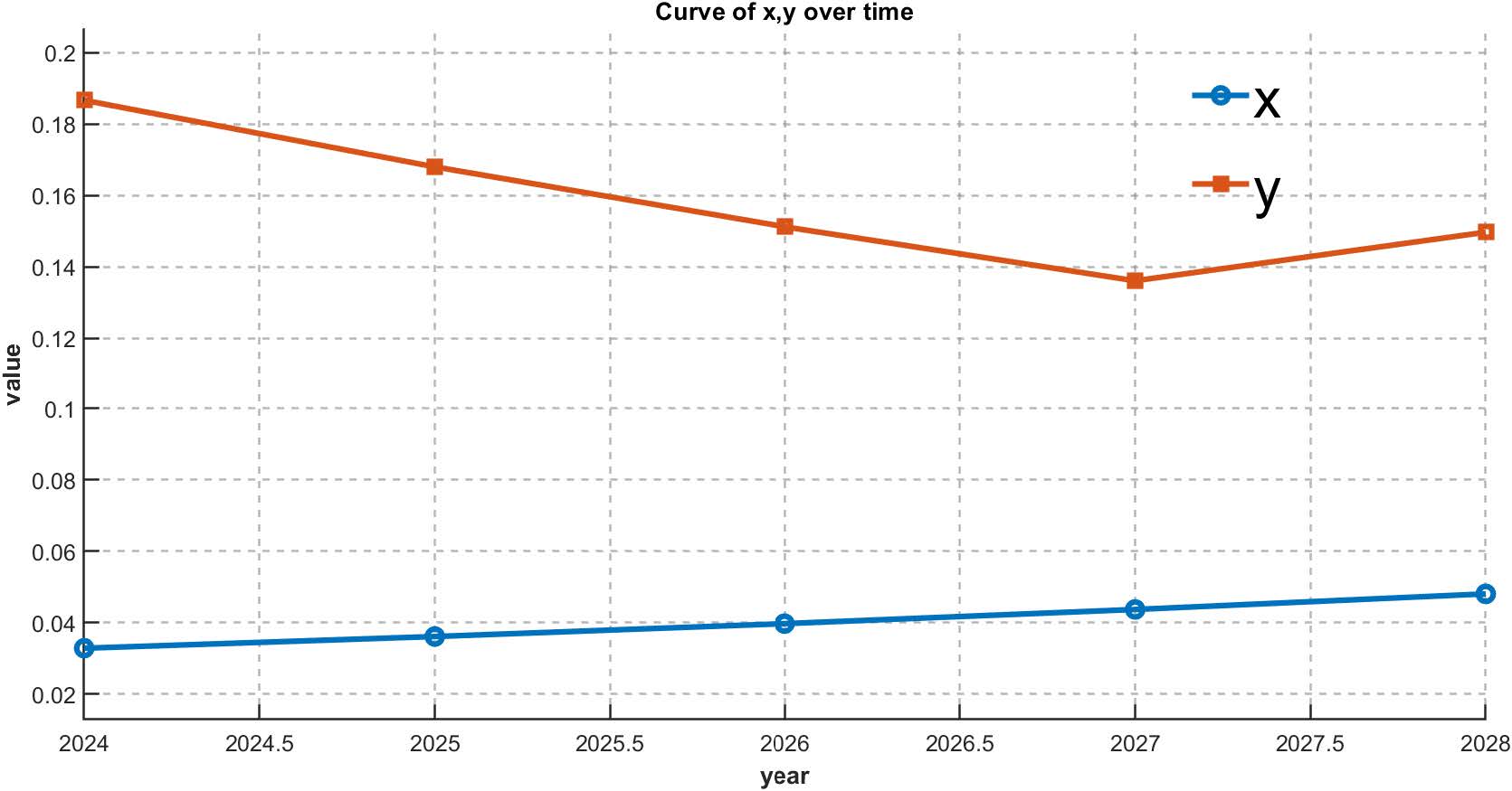
Figure 12: Curve of x, y over Time
Through these two graphs, we find that the Juneau government in 2025 if it makes x increase by increasing the cost of tourism and restricting the purchase of alcohol, therefore leading to a decrease in tourism, so the environmental index of the city of Juneau increases dramatically, but this also leads to a decrease in the tourist audience of the city of Juneau and weakening of the economic benefits and decrease in the level of satisfaction of the inhabitants. However, this situation will not last for a long time and the Juneau City government can actively develop other sectors such as services and mining. A small increase in tourist arrivals is expected after 2027, which will lead to economic growth and a rebound in resident satisfaction, easing social pressures.
5. Sensitivity Analysis
5.1 Sensitivity Analysis Overview
In what follows, we will perform a partial sensitivity analysis and a global sensitivity analysis of this model we have built above respectively, to determine the effect of the change in the magnitude of the change in our final optimization objective D(x,y) caused by a change in the independent variable x,y.
5.2 Partial Sensitivity Analysis of the FunctionD(x,y) near the Point of Maximum Value
In this part, we compute the partial sensitivity of D(x,y) near the point of maximum using a function taking partial derivatives. (equation 29)
separate calculations give us:
So we find: near the extreme point, each 1% increase of x,the optimization objective D(x,y) decreases by 6.36%,and each 1% increase ofy,the optimization objectiveD(x,y) decreases by 3.30%. It can be seen that the small change ofx,y has little effect on the optimization objectiveD(x,y), which is negligible.
5.3 Global Sensitivity Analysis of the FunctionD(x,y) Based on Monte Carlo Simulation
In this part, we examine the sensitivity relationship of the maximum point to the global. We use Monte Carlo simulation to obtain the distribution image of EcI,EnI,S by randomly selecting 100 sample points each from the resultingEcI,EnI,SI,(figure 13)
These data were then brought into our objective optimization function D(x,y) to obtain an image of the distribution of its values.(figure 14).
It is observed that the mean value of coordination is 0.3524 while the extreme values of the data are 0.328, 0.377 respectively. they deviate from the mean value by 6.923%, 6.981% and the extreme deviation is only 0.049. it is evident that the treatment of this model has less impact on the final result and is reasonable and convincing.
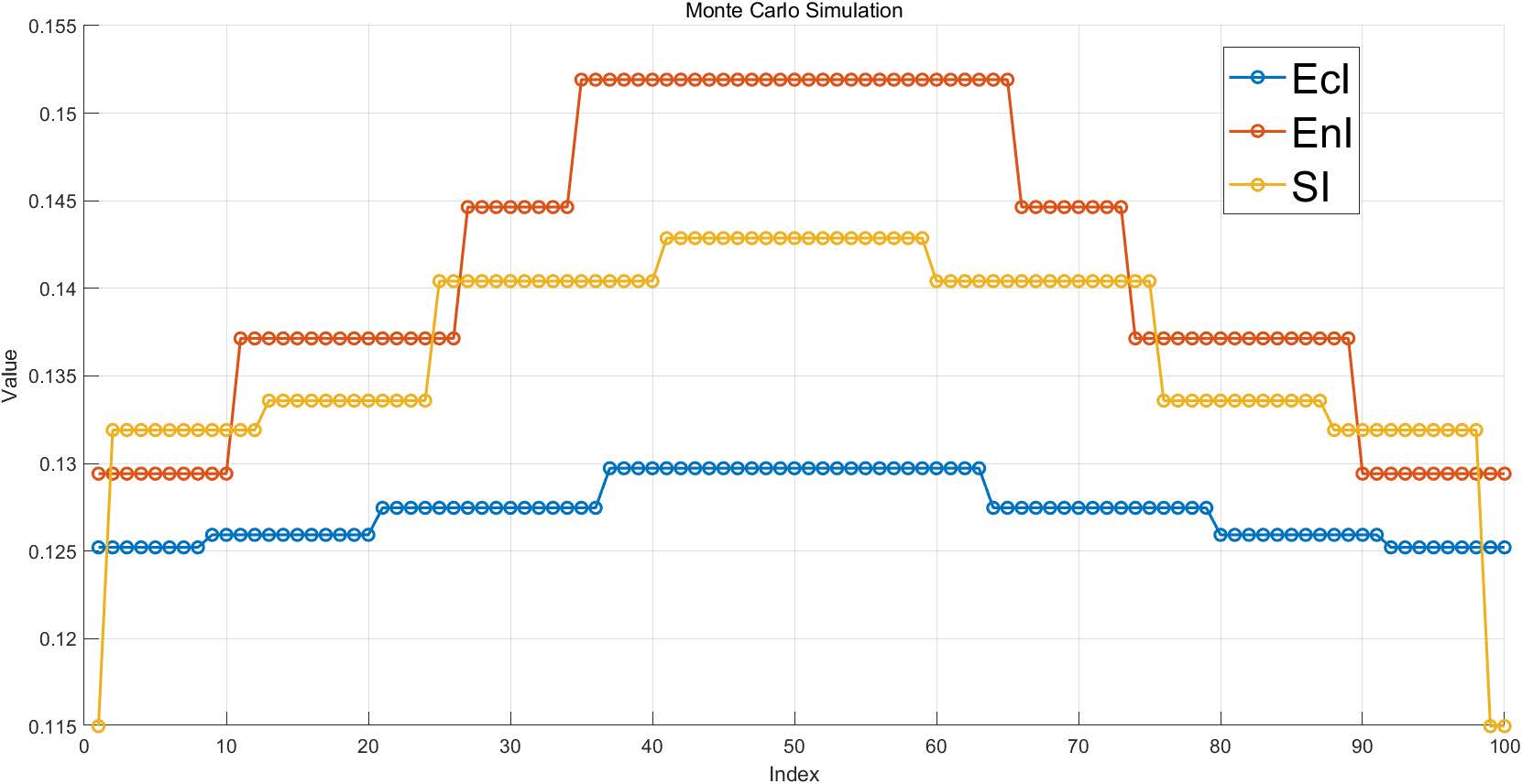
Figure 13: Monte Carlo Simulation
Figure
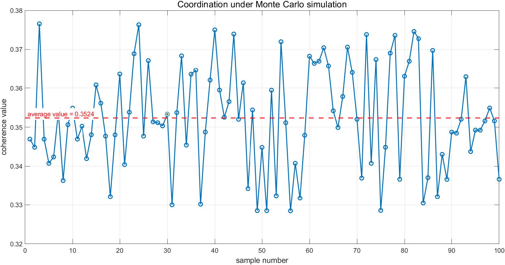
Figure 14: Coordination Degree D(x, y) under Monte Carlo Simulation
6. Application of the Model: Optimizing Sustainable Tourism Plans in OtherWorld Tourist Cities
6.1 Hawaii with Over-tourism
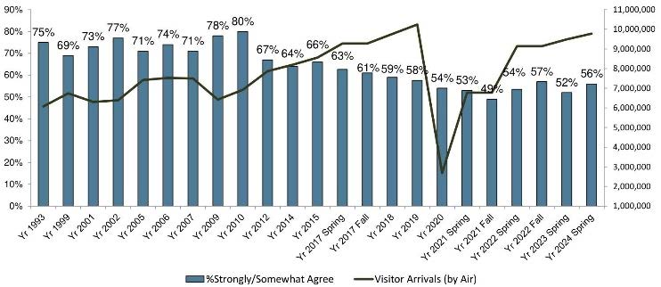
Hawaii has long faced the problem of “over-tourism”, with the number of tourists exceeding 10 million in 2019 (the local population is only about 1.5 million), resulting in enormous pressure on the ecosystem and the lives of the residents. Popular attractions such as Hanauima Bay, where the influx of tourists has led to coral deaths and deteriorating water quality, have recovered dramatically after the decline in visitors during the epidemic, highlighting the damage done to nature by tourism activities. Local residents face housing shortages, water stress, and infrastructure overload, and nearly half of residents in 2020 believe that tourism does more harm than good.Although Hawaii has adopted management measures such as reservation systems, limiting the number of tourists, increasing non-resident fees, and imposing 'green fees', tourism remains an economic pillar, and balancing economic benefits with sustainable development remains a challenge. Therefore, we apply our model to Hawaii to realize the sustainable development of Hawaii's tourism industry.
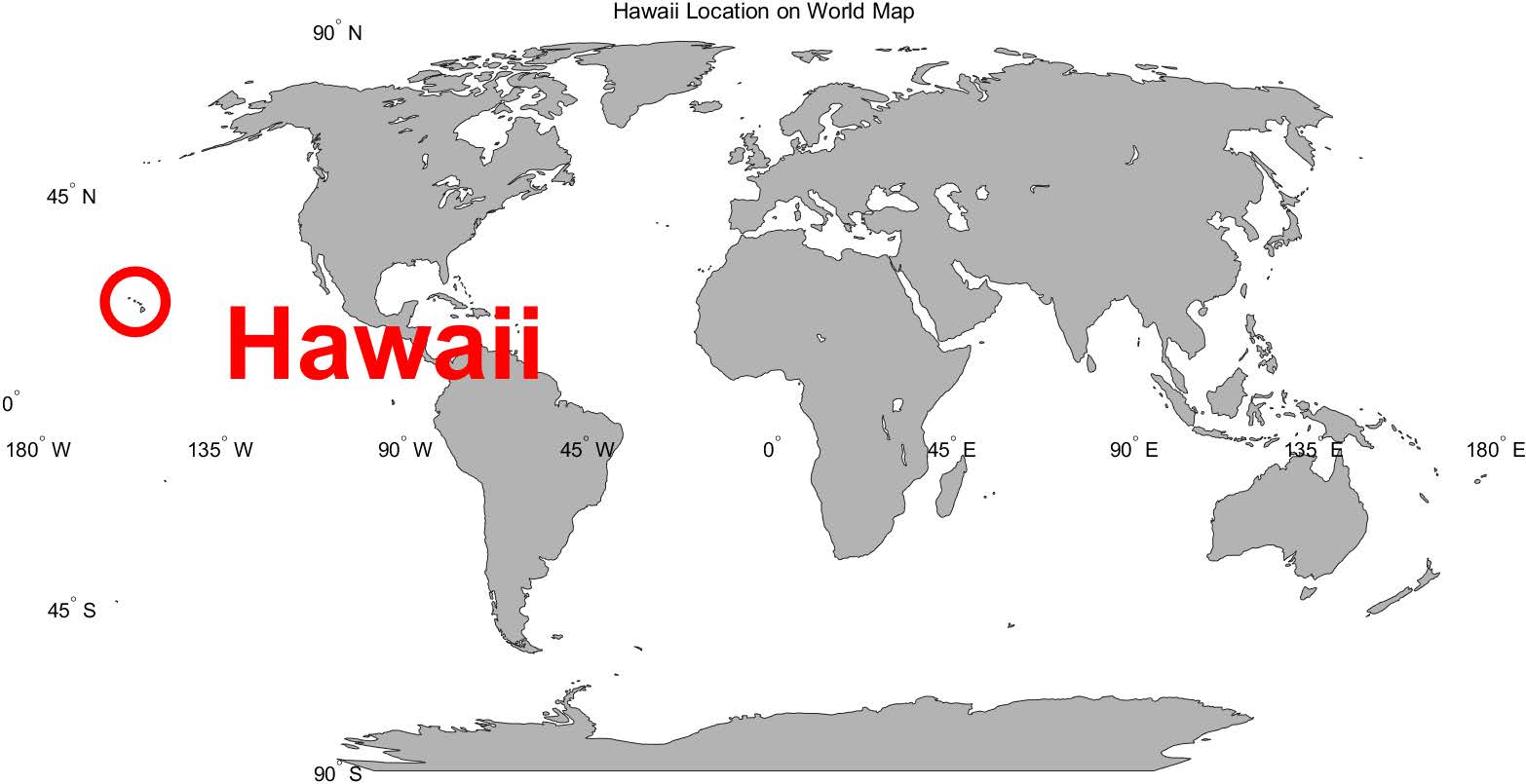
Figure 15: Geographic Location of Hawaii

Figure 16: The View from Hawaii
Based on our coupled coordination degree model, we analyze and calculate the coupled coordination degree of Hawaii's tourism in terms of economic, environmental, and social aspects to assess the impacts of relevant measures in the current tourism situation in Hawaii, and to give a reasonable strategy for future tourism development.
Unlike the previous study of Juneau, Alaska, we quantitatively assessed the dynamic reality of the environment by using the local AQI (Air Quality Index) index(figure 17.as the environmental index for the past years. We also quantitatively assessed the impacts of the environmental measures on the current tourism situation in Hawaii by analyzing and calculating the degree of coupled coordination between economic aspects and social aspects.
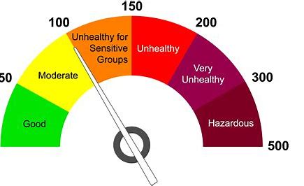
Figure 17: Air Quality Index
On the social side, we quantified the social satisfaction index index based on local polls over the years on the pros and cons of the impact of Hawaii's tourism industry on the local area, and then determined the social satisfaction index index accordingly.
Same as the previous city of Juneau, Alaska, we also used the number of tourists x and the rate of increase in tourist fees y as decision variables.The following table (tourist arrivals in 10,000, per capita consumption in $10, environmental/social satisfaction index in no unit) is obtained after summarizing all the raw data:
We refer to equation(1)(4)(5)(6), and utilize the same method as the data processing for the city of Juneau to progressively generalize the expression for T in the form of equation 13, and then refer to the fitted formulas utilizing(14)(15)(17)(18) to progressively generalize the fitted eni expression eni skimming in the form of equation (16)and the s skimming expression in the form of equation (19):
By using the above expressions for EnI''(x,y) and SI''(x,y), after retaining the digits appropriately, the expression on T in the shape of equation (20) is summarized:
Finally, we generalize the expression for D''(x,y) according to equation (21)(22):
included among these:
Like equation 23 , Hawaii also has a constraint on the number of visitors:Hawaii has to have less than 12,000,000 visitors,which is satisfied because of the normalization process:
which is finally calculated:
Based on the above results we conclude that measures should be taken to keep consumption growth around 3% and the number of tourists should be kept at the corresponding value of 9936000 before normalization of y.
6.2 Detroit with Prospects for Tourism Development
With its deep cultural heritage and unique industrial legacy, Detroit, USA, has significant tourism potential that has yet to be fully realized. As the birthplace of the “Motor City” and “Motown Music”, Detroit is home to cultural landmarks such as the Henry Ford Museum and Motown Museum, as well as pioneering street art such as the Heidelberg Art Project, attracting art and history lovers. However, with only 970 thousand visitors in 2023, the region's lack of infrastructure, limited international visibility, and lagging development of sustainable tourism continue to constrain its emergence as a mainstream tourist destination.
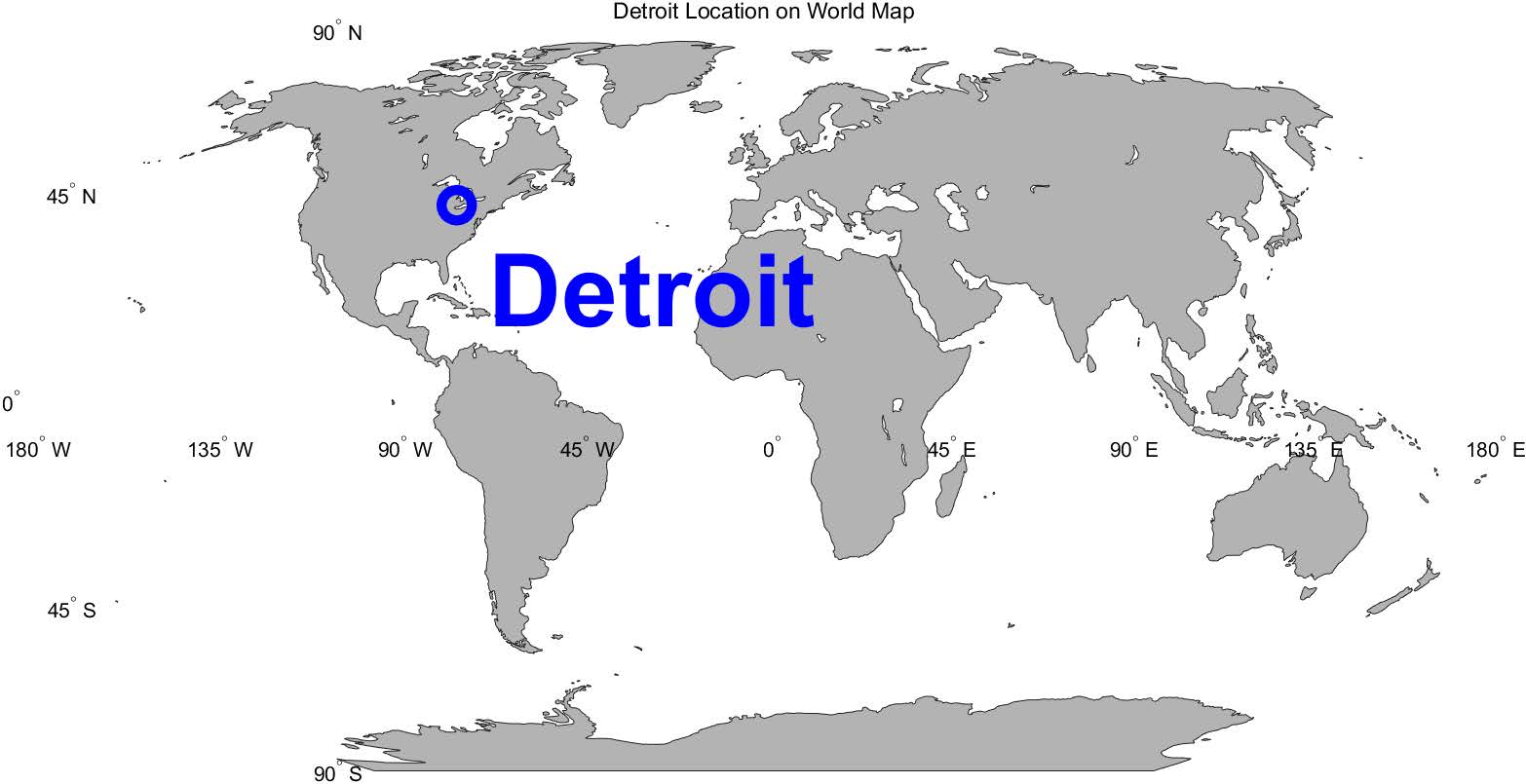
Figure 20: Geographic location of Detroit

Figure 21: The View from Detroit
Also based on our coupled coordination model, we analyze and calculate the degree of coupled coordination between the economic, environmental and social aspects of tourism in Detroit to assess the current situation of Detroit and give recommendations and methods for developing tourism. For Detroit, we also choose the total economic data of tourism as the economic indicator.Due to the specificity of Detroit's environment, we do not only choose the AQI index as the environmental index, but also add the green coverage rate as a factor that affects the environmental index based on the AQI index.Lastly, we measured the resident satisfaction index by the data of per capita income and employment rate.
Processing and operating the data according to the model, we get the following calculation: when the tourist population reaches 2.5 million people and the per capita tourist consumption decreases by about 5%, the coupling of the parties reaches the best state.
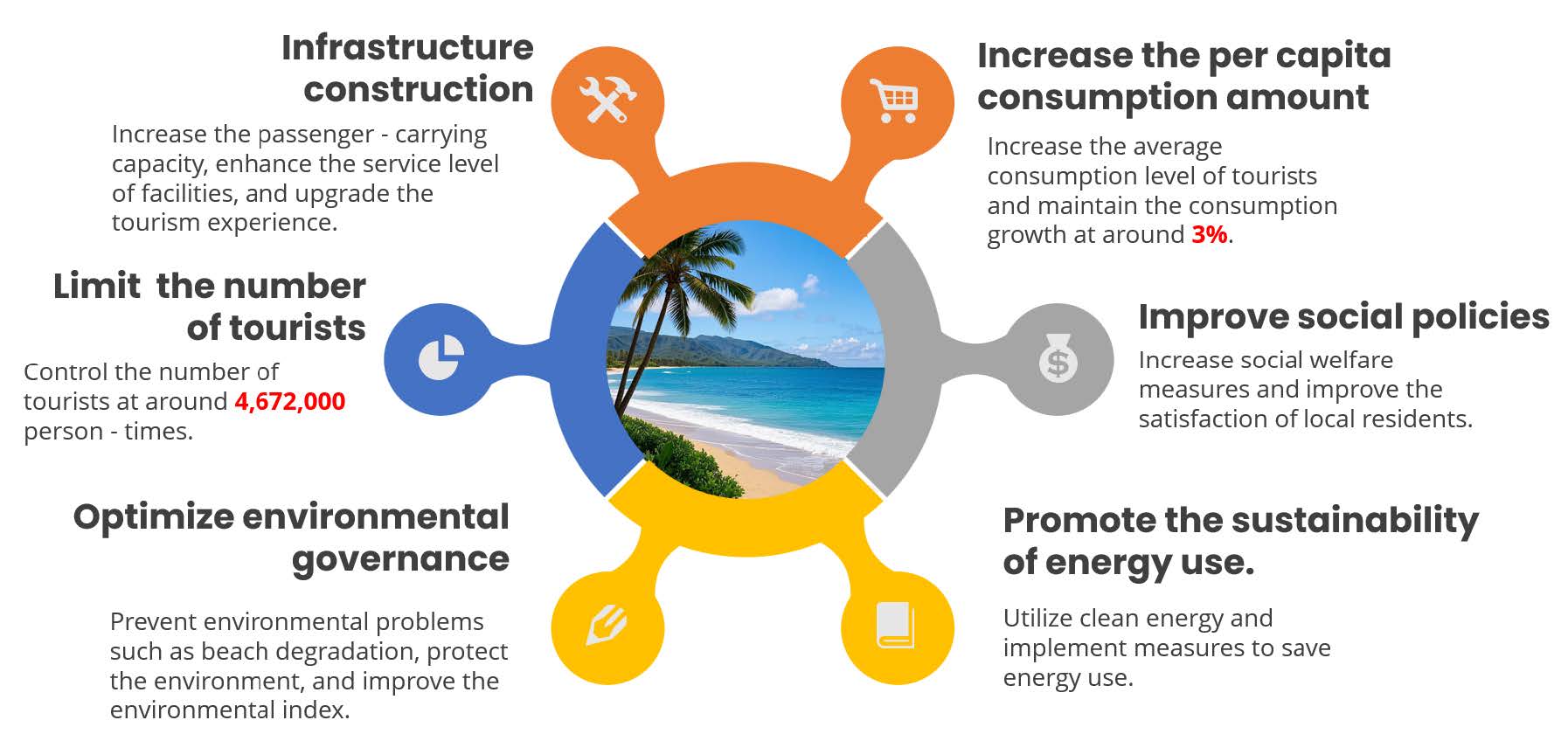
Figure 22: Hawaii Tourism Development Strategy
7. Model Evaluation
7.1 Strengths
The model is more generalizable and can be applied not only to over-touristed cities like Juneau, but also to potential tourist attractions like Detroit and give corresponding policies.
The model is analyzed by sensitivity analysis, which proves the validity and accuracy of the model, and can better characterize the magnitude of the impact of policy changes.
The model is able to accurately give the government's funding allocation and future trends of each indicator, and has a good prediction function.
7.2 Weeknesses
The independent variables of this model only consider the rate of increase in tourism spending and the maximum number of tourists, without considering other potential influencing factors.
This model is a reasonable function solution rather than an optimal solution obtained by fitting regression, so the maximum value obtained has a slight error with the actual situation.
8. Conclusions
In the part of coupling coordination degree model building: we established the comprehensive evaluation index T related to economy, environment and society, and found that social satisfaction index is mainly affected by house price and poverty rate by using principal component analysis-factor analysis. The weights of carbon emission and glacier area in the environmental index were determined to be 0.4976 and 0.5024 by entropy weighting method, and the weights of house price and poverty rate in the social satisfaction index were 0.7794 and 0.2206, respectively, and the weights of the economical index, the environmental index, and the social satisfaction index in the comprehensive evaluation index were 0.3152, 0.1936, and 0.4912, respectively.The model building part of the model was established through the fitting regression, we established the functional relationship between the environmental and social indexes and the maximum number of tourists and the growth rate of average tourist consumption, and obtained the optimal solution of the static model: when the maximum number of tourists is 1,175,000, and the average consumption of tourism is increased by 2.98%, the coupling degree of the three systems is the best. Finally, we plan to allocate funds according to the weights, and use the time series model to predict the impact of environmental protection on social satisfaction in 2024-2027 and the driving effect of a small increase in the number of tourists on the economy and residents' satisfaction after 2027.
In the Inspiration Analysis part:we proved the validity of the model through local and global sensitivity analysis and pointed out that the increase rate of average tourist spending is the key influencing factor.
In the model citation part: we selected Hawaii, which is over-touristed, and Detroit, which is yet to be developed. In Hawaii, combined with the characteristics of tropical islands, it is calculated that the coupling of the three indicators peaks when consumption increases by about 3% and the number of tourists is controlled at 4,672,000. It is suggested to raise the hotel tax to promote tourist consumption, and allocate the tax revenue to infrastructure development (65.39%), environmental protection (26.6%), and social welfare (8.01%) according to weights for optimization. In Detroit, calculations show that the combined benefits and the coupling of the three indicators are optimal when there are 2.5 million tourists and consumption is reduced by about 5%. It is recommended to reduce or waive part of the tourism tax, dig deeper into local resources, and promote the healthy and rapid development of the tourism industry.
In summary, we suggest that the Juneau government actively engage in environmental protection and reasonably allocate funds according to weights to help the sustainable development of the tourism industry.
9. References
[1] Alaska Coastal Rainforest Center (ACRC), Juneau climate report: Juneau’s changing
climate & community response, https://acrc.alaska.edu/juneau-climate-report/.
[2] R. Pinyang, B. Peipei, and G. Yaxin, “Tourism community farmers’ livelihood adapt-
ability response in the process of rural revitalization —— a two - way coupling
model based on ecological service dependence and livelihood well - being,” Tourism
and Hospitality Research, vol. 24, no. 1, pp. 66–79, 2024.
[3] shangchuanba.com, Juneau restricts cruise ship passenger arrivals, https : / / www.
shangchuanba.com/company/article/300552604, 2024.
[4] G. T. News, Hawaii is seriously overloaded. can the pandemic cure ’over - tourism’? https://www.traveldaily.cn/article/146300.
[5] Pre - generated data files, https://aqs.epa.gov/aqsweb/airdata/download_files.
html#eighthour.
[6] O. Group, Resident sentiment survey 2024, https://www.hawaiitourismauthority.
org/media/13071/resident-sentiment-spring-2024.pdf.
[7] Annual visitor research reports, https://www.hawaiitourismauthority.org/research/
annual-visitor-research-reports/.
[8] Tourism data, https://dbedt.hawaii.gov/visitor/tourismdata/.
[9] Guide of US, LLC, Hawaii tourism statistics, https : / / www. hawaii - guide . com /
hawaii-tourism-statistics.
[10] Detroit tourism statistics, https://www.connollycove.com/detroit-tourism-statistics/.
[11] Visit detroit - official tourism site, https://visitdetroit.com/.
[12] Green infrastructure - detroit water and sewerage department, https://detroitmi.gov/
departments/detroit-water-and-sewerage-department/green-infrastructure.
[13] Detroit, mi - bureau of labor statistics, https://www.bls.gov/regions/midwest/mi_
detroit.htm
10. MEMORANDUM
To: Juneau City Council Leaders From: MCM Team 2525898 Date: February 17, 2025
In order to achieve the goal of sustainable development in the City of Juneau, we recommend that business taxes be adjusted for both local and foreign businesses, and that tax rates be increased moderately, especially for tourism-related industries (hotels, attractions, transportation, etc.), to be used to supplement tourism-specific funding. Appropriately increase the price of tourism tickets according to the low and high seasons of tourism to regulate the flow of tourists and increase revenue. Appropriately limit the consumption of alcoholic beverages and food and beverage by tourists during peak seasons to reduce the waste of resources, ease the pressure on the food and beverage industry, advocate green consumption patterns, and encourage the consumption of local specialty drinks and food. Meanwhile, in order to stabilize the social situation, the annual limit on the number of tourists and tourism funding should not be raised by more than 10%. Secondly, it should be dynamically adjusted year by year to optimize the combination of measures year by year according to the analysis results of the dynamic planning model.
2025-2027: Focus on environmental protection, with constant small increases in taxes and reductions in the number of tourists during this period to achieve a reduction in carbon emissions and mitigate the challenges of receding glacier lengths.
2027 and beyond: Based on market feedback, gradually improve the price adjustment mechanism, appropriately increase the number of passengers, reduce taxes, and expand the scope of the policy of limiting consumption, which will lead to socio-economic development and improve the well-being of the people, to ensure that the optimization of the long-term effect.
Our forecast suggests that the City of Juneau should try to limit the number of annual visitors to 1,175,000 through the above measures to reduce the pressure on the city's infrastructure; at the same time, tourism funding should be increased by 2.98% to provide more support for municipal construction and tourism industry upgrades.
The Juneau City Council should spend 19.36% of the funding revenue on encouraging businesses and factories, 31.52% on reforestation and carbon reduction retrofitting of mining factories, and 49.12% on improving infrastructure to ensure the long-term sustainability of the city's tourism industry.
We believe that the implementation of the above measures will strike a balance between enhancing tourism revenues and promoting environmental protection, while bringing a brighter future to Juneau's tourism industry.
We look forward to the Juneau City Council considering the above recommendations and moving forward with the implementation of the relevant policies. For further support, we are ready to provide more detailed analysis and adjustments to the dynamic planning model.